Parallel algorithms for studying the system of long Josephson junctions

Параллельные алгоритмы для исследования системы длинных джозефсоновских переходов*

M.V. Bashashin^1,3, A.V. Nechaevskiy¹, D.V. Podgainy¹, I.R. Rahmonov², Yu.M. Shukrinov^2,3, O.I. Streltsova^1,3, E.V. Zemlyanaya^1,3, M.I. Zuev¹
¹Laboratory of Information Technologies JINR
²Bogoliubov Laboratory of Theoretical Physics JINR
³Dubna State University

*The study was supported by the Russian Science Foundation (the project № 18-71-10095).

The results on studying the efficiency of parallel implementations of the computing scheme for calculating the current-voltage characteristics of the system of long Josephson junctions are presented in the paper [1-4]. The following parallel implementations were developed: the OpenMP implementation for computing on systems with shared memory, the CUDA implementation for computing on NVIDIA graphics processors. The development, debugging and profiling of parallel applications were performed on the education and testing polygon of the HybriLIT heterogeneous computing platform, while calculations were carried out on the GOVORUN supercomputer [2].

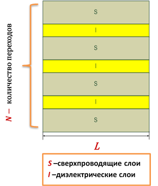Formulation of the problem. A generalized model that takes into account the inductive and capacitive coupling between long Josephson junctions (LJJ) is considered [1]. The system of coupled LJJ is supposed to consist of superconducting and intermediate dielectric layers with a length L.

The phase dynamics of the system N LJJ taking into account the capacitive and inductive coupling between the contacts is described by the initial-boundary problem for the system of differential equations relative to the difference of phases $\phi _{l}(x,t)$ and voltage $V _{l}(x,t)$ at each $l$ contact ( $l=1,2,...N$ ). In a dimensionless form, the system of equations has the form [1]:

$\left\{\begin{matrix} \frac{\partial \phi }{\partial t}& = C\cdot V, 0<x<L,t>0\\ \frac{\partial V }{\partial t}& =L^{_{-1}}\frac{\partial^2\phi }{\partial x^2}-\beta V-sin(\phi )+I(t); \end{matrix}\right.$

$\phi =\begin{pmatrix} \phi_{1}\\ \phi_{2}\\ \cdot \cdot \cdot \\ \phi_{N}\\ \end{pmatrix}, V =\begin{pmatrix} V_{1}\\ V_{2}\\ \cdot \cdot \cdot \\ V_{N}\\ \end{pmatrix},$

where L — is the inductive coupling matrix, С — is the capacitive coupling matrix:

$L=\begin{pmatrix} 1& S& 0& \cdots& \square& 0& S \\ \vdots& \vdots& \vdots& \vdots& \vdots& \vdots& \vdots&\\ \cdots& 0& S& 1& S& 0& \cdots&\\ \vdots& \vdots& \vdots& \vdots& \vdots& \vdots& \vdots&\\ \square& \square& \square& \square& \square& \square& \square& \\ S& 0& \cdots& \cdots& 0& S& 1& \end{pmatrix}, C=\begin{pmatrix} D^{C}& S^{C}& 0& \cdots& \cdots& 0& 0& S^{C}&\\ \vdots& \vdots& \vdots& \vdots& \vdots& \vdots& \square& \vdots&\\ \cdots& 0& S^{C}& D^{C}& S^{C}& 0& \cdots& \cdots&\\ \vdots& \vdots& \vdots& \vdots& \vdots& \vdots& \vdots& \vdots&\\ \cdots& \cdots& \cdots& \cdots& 0& S^{C}& D^{C}& S^{C}&\\ S^{C}& 0& \cdots& 0& S^{C}& 0& S^{C}& D^{C}& \end{pmatrix},$

β — is the dissipation parameter, the inductive coupling parameter S takes a value in the interval 0<|S |<0.5; D ^c— is the effective electric JJ thickness normalized by the thickness of the dielectric layer; s_c — is the capacitive coupling parameter, $l(t)$ — is the external current.

The system of equations is supplemented with zero initial and boundary conditions:

$V_{l}(0,t)=V_{l}(L,t)=\frac{\partial \phi (0,t)}{\partial x}=\frac{\partial \phi (L,t)}{\partial x}=0, l=1,2,...,N.$

The problem when boundary conditions in the direction x were defined by the external magnetic field was also considered [2].

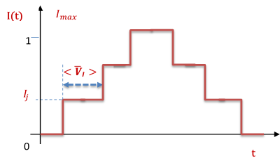
When calculating the current-voltage characteristics (CVC), the dependence of the current on time was selected in a form of steps (a schematic presentation is given in the figure below), i.e. the problem is solved at the constant current ( $I=I_{j}$ ), while the found functions $\phi_{l},V_{l}(l=1,2,...N)$ are taken as initial conditions to solve the problem for the current $I_{j+1}$ .

Computing and parallel schemes. For the numerical solution of the initial-boundary problem, a uniform grid by the spatial variable (the number of grid nodes NX ). was built. In the system of equations (1) the second-order derivative by the coordinate x is approximated using three-point finite-difference formulas on the discrete grid with a uniform step $\Delta x$ . The obtained system of differential equations relative to the values $\phi_{l},V_{l}(l=1,2,...N)$ in the nodes of the discrete grid by x is solved by the fourth-order Runge-Kutta method.

To calculate CVC the averaging $V_{l}(x,t)$ over the coordinate and time is performed. To do this, at each time step, the integration of voltage over the coordinate using the Simpson method and the averaging are carried out

$\bar{V_{l}}=\frac{1}{L}\int_{0}^{L}V_{l}(x,t)dx,$

then the voltage is averaged over time using the formula

$<\bar{V_{l}}>=\frac{1}{T_{max}-T_{min}}\int_{T_{min}}^{T_{max}}\bar{V_{l}}(t)dt$

and summed by all JJ. To integrate over time, the rectangle method is used.

Parallel scheme. While numerically solving the initial-boundary problem by the fourth-order Runge-Kutta method over the time variable, at each time layer the Runge-Kutta coefficients ( $K_{i}$ ) can be found independently (in parallel) for all NX nodes of the spatial grid and for all N Josephson junctions. Meanwhile the coefficients $K_{i}(i=1,2,3,4)$ are defined one by one (sequentially). Thus, the parallelization is effectively performed on $NX \cdot N$ points. When carrying out the averaging in CVC computing, the calculation of integrals can be performed in parallel as well.

Parallel implementations. To speed up CVC computing, parallel implementations of the computing scheme described above were developed. The results on studying the efficiency of parallel implementations performed at the values of the following parameters: $L=10;I_{min}=0;I_(max)=1.1;\beta=0.2;N=1;$ $T_(max)=200; \Delta t=0.04$ — are presented below; the number of nodes by the spatial variable is:

NX = 20048.

OpenMP implementation.
The calculations were performed:

on computing nodes with the processors Intel Xeon Phi 7290 (KNL: 16GB, 1.50 GHz, 72 core, 4 threads per core supported — total 288 logical cores), the compiler Intel (Intel Cluster Studio 18.0.1 20171018);
on dual-processor computing nodes with the processors Intel Xeon Gold 6154 (Skylake: 24.75M Cache, 3.00 GHz, 18 core, 2 threads per core supported — total 72 logical cores per node).

The graphs of the dependence of the calculation speedup obtained using the parallel algorithm:

$S=\frac{T_{1}}{T_{n}};$

where $T_{1}$ is the calculation time using one core, $T_{n}$ — is the time of calculations on $n$ -logical cores, on the number of threads, the number of which is equal to the number of logical cores, and the graph of the dependence of efficiency of using computing cores by the parallel algorithm:

$E=\frac{T_{1}}({n\cdot T_{n})}\cdot100 \% .$

characterizing the scalability of the parallel algorithm, are presented below.

Fig. 1 and Fig. 2 show the dependence of speedup and efficiency on the number of threads when performing calculations on the nodes with the processors Intel Xeon Phi, while Fig. 3 and Fig. 4 illustrate the dependence of speedup and efficiency when applying the possibility to use the instruction AVX-512. It is noteworthy that the use of this instruction allowed us to reduce the calculation time in 1.8 times.

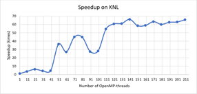
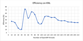
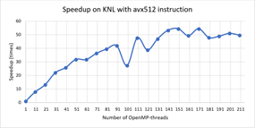
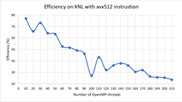
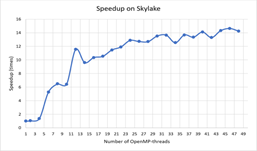
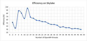
Fig. 3. Graph of the dependence of **speedup** of parallel computing on the number of threads. Compilation of the program with the option -xMIC-AVX512

Fig. 4. Graph of the dependence of **efficiency** of using computing nodes by the parallel algorithm on the number of threads. Compilation of the program with the option -xMIC-AVX512

Fig. 5 and Fig. 6 show the dependence of speedup and efficiency on the number of threads when performing calculations on the nodes with the processors Intel Xeon Gold 6154.

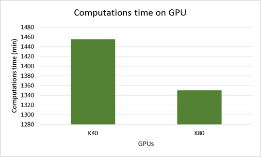
CUDA implementation. A CUDA implementation of the parallel algorithm was developed for computing on NVIDIA graphics accelerators. The parallel reduction algorithm using shared memory was applied for calculating integrals. The calculation time on the graphics accelerators Nvidia Tesla K40 and Nvidia Tesla K80 is presented in the diagram below.

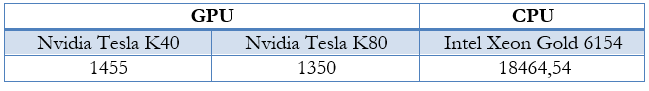
Comparative analysis of parallel implementations. Table 1 shows the results of the minimum calculation time obtained on various computing architectures.

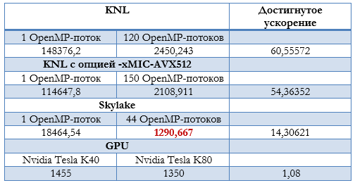
Table 2. Calculation time (in minutes) on 1 OpenMP thread of the Skylake processor and on the graphics accelerators Nvidia Tesla K40 and Nvidia Tesla K80

The best (minimum) time for the above values of the parameters to calculate CVC of LJJ is 1290 minutes; it was achieved in calculations on the dual-processor node with the processors Intel Xeon Gold 6154.

[1] P. H. Atanasova, M.V. Bashashin, I.R. Rahmonov, Yu.M. Shukrinov, E.V. Zemlyanaya. Influence of the inductive and capacitive coupling on the current-voltage characteristic and electromagnetic radiation of the system of long Josephson junctions. Journal of Experimental and Theoretical Physics, Vol. 151, № 1, pp. 151-159, in Russian (2017)

[2] Gh. Adam, M. Bashashin, D. Belyakov, M. Kirakosyan, M. Matveev, D. Podgainy, T. Sapozhnikova, O. Streltsova, Sh. Torosyan, M. Vala, L. Valova, A. Vorontsov, T. Zaikina, E. Zemlyanaya, M. Zuev. IT-ecosystem of the HybriLIT heterogeneous platform for high-performance computing and training of IT-specialists. CEUR Workshop Proceedings (CEUR-WS.org) (2018 г.)

[3] Bashashin M.V., Zemlyanay E.V., Rahmonov I.R., Shukrinov J.M., Atanasova P.C., Volokhova A.V. Numerical approach and parallel implementation for computer simulation of stacked long Josephson Junctions. Computer Research and Modeling, 2016, vol. 8, no. 4, pp. 593-604

[4] E. V. Zemlyanaya, M. V. Bashashin, I. R. Rahmonov, Yu. M. Shukrinov, P. Kh. Atanasova, and A. V. Volokhova, Model of stacked long Josephson junctions: Parallel algorithm and numerical results in case of weak coupling. AIP Conference Proceedings, vol 1773, 110018, (2016)

Download pdf-file